In part 1 , we looked at the theory behind Q-learning using a very simple dungeon game with two strategies: the accountant and the gambler. This second part takes these examples, turns them into Python code and trains them in the cloud, using the Valohai deep learning management platform.
Due to the simplicity of our example, we will not use any libraries like TensorFlow or simulators like OpenAI Gym on purpose. Instead we will code everything ourselves from scratch to provide the full picture.
All the example code can be found at https://github.com/valohai/qlearning-simple
Code Layout
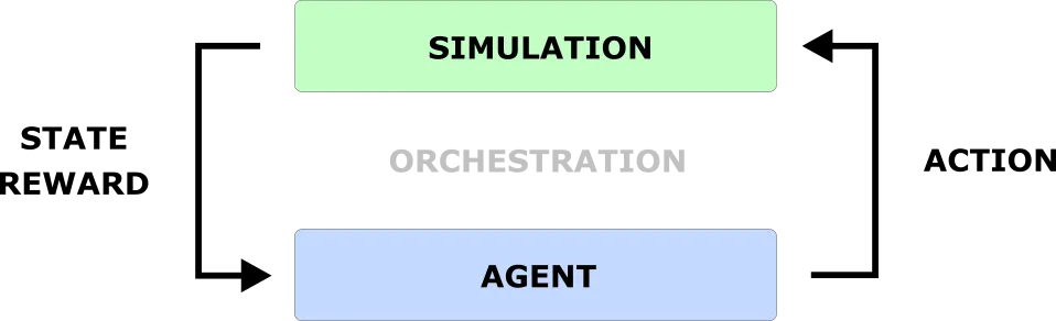
A typical reinforcement learning codebase has three parts:
- Simulation
- Agent
- Orchestration
Simulation is the the environment where the agent operates. It updates state and hands out rewards, based on its internal rules and actions performed by the agent(s).
Agent is an entity operating in the simulation, learning and executing a strategy. It performs actions, receives state updates with rewards and is learning a strategy to maximize them.
Orchestration is all the rest of the boilerplate code. Parsing the parameters, initializing environment, passing data between the simulation and the agents and finally closing the shop down.
Simulation
We will use the dungeon game introduced in the part 1. These are the rules:
- The dungeon is 5 tiles long
- The possible actions are FORWARD and BACKWARD
- FORWARD is always 1 step, except on last tile it bumps into a wall
- BACKWARD always takes you back to the start
- Sometimes there is a wind that flips your action to the opposite direction
Unknown to the agent:
- Entering the last tile gives you +10 reward
- Entering the first tile gives you +2 reward
- Other tiles have no reward
Agent
In the first part of the tutorial , we introduced two strategies: The accountant and the gambler. The accountant only cared about past performance and guaranteed results. The gambler was more eager to explore riskier options to reap bigger rewards in the future. That said, to keep the first version simple, the third strategy is introduced: The drunkard.
The drunkard is our baseline strategy and has a very simple heuristic:
- Take random action no matter what
Orchestration
Now that we have our simulation and the agent, we need some boilerplate code to glue them together.
Dungeon simulation is turn-based so the flow is simple:
- Query the agent for next action and pass it to the simulation
- Get the new state and reward back and pass them to the agent
- Repeat
Infrastructure
While it is possible to run simple code like this locally, the goals is to provide an example of how to orchestrate more complicated project properly.
Machine learning is not equal to software development. Just pushing your code to a Git repository is not enough. For full reproducibility, you need to version control things like data, hyperparameters, execution environment, output logs and output data.
Running things locally also slows you down. While toy examples often give a false sense of fast iteration, training real models for real problems is not a suitable task for your laptop. After all, it can only run one training execution at a time, where a cloud-based environment lets you start dozens simultaneously with fast GPUs, easy comparison, version control and more transparency toward your colleagues.
Valohai Setup
Head out to valohai.com and create an account. As a default, you’ll have 10$ worth of credits on your account which is enough for running the following trainings on cloud instances.
After you are signed up, click skip tutorial or open the Projects dropdown from the top-right and select Create project .
Name your project something meaningful and click the blue Create project button below.
We already have our code and valohai.yaml in the example git repository at https://github.com/valohai/qlearning-simple.
We just need to tell Valohai where they are, too. Click the project repository settings link shown in the screenshot above or navigate to Settings > Repository tab.
Paste the repository url in the URL field, make sure Fetch reference is “master” and then click Save .
Execute!
Everything is in place so it is time for our first execution.
Click the big blue Create execution button In the Valohai project Executions tab.
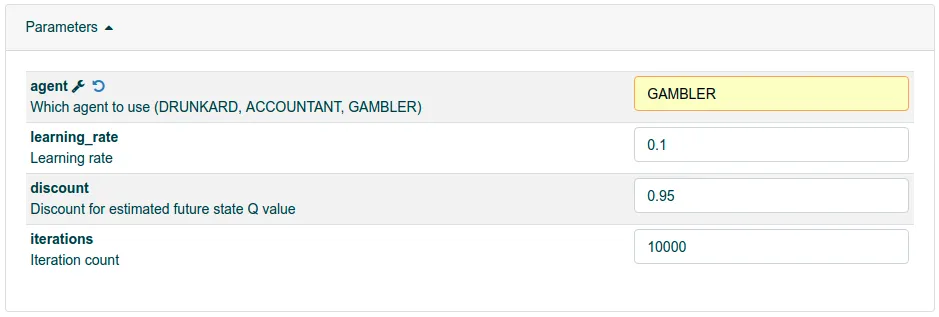
The valohai.yaml file from our Git repository has provided us with all the right defaults here. If you want to know more about valohai.yaml, check out the documentation .
Go ahead and click the blue Create execution button in the bottom.
Running an execution in Valohai means that roughly the following sequence will take place under the hood:
- New server instance is started
- Your code and configuration (valohai.yaml) is fetched from a git repository
- Training data is downloaded
- Docker image is downloaded and instantiated
- Scripts are executed based on valohai.yaml + your parameters
- All stdout is stored as log + JSON formatted metadata is parsed for charts
- Entire environment is version controlled for reproducibility later on
- The server instance is shut down automatically once the script(s) are done
Isn’t it amazing what you can get with just a single mouse click!
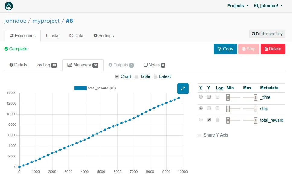
If you head out to the Metadata tab of the execution, you can see how our agent with the DRUNKARD strategy has collected rewards. Not surprisingly, the strategy of taking random actions will produce almost a straight line with a slight wobble, which informs us that no learning is taking place.
The Accountant
After running the baseline random strategy, it is time to bring back the two original strategies introduced in the part 1 of the tutorial : The accountant and the gambler.
The accountant has the following strategy:
- Always choose the most lucrative action based on accounting
- If it is zero for all options, choose a random action
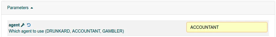
To execute the ACCOUNTANT, remember to change the agent parameter for your execution and then click the blue Create execution again.
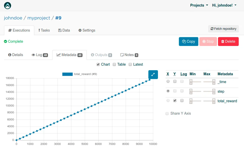
Looking at the Metadata tab, the accountant isn’t much better in terms of learning. The curvature is even straighter, because just after first few iterations, it will learn to always choose BACKWARD for the consistent +2 reward and not wobble like the random drunkard.
The total reward is about +4000 higher, though. Some improvement at least!
The Gambler
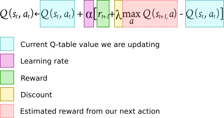
From our three agents, the gambler is the only one doing real Q-learning. Remember our algorithm from the part 1 :
The strategy is as follows:
- Choose the most lucrative action from our Q-table by default
- Sometimes gamble and choose a random action
- If the Q-table shows zero for both options, choose a random action
- Start with 100% gambling (exploration), move slowly toward 0% (exploitation)
Again remember to change the agent from your parameters listing!
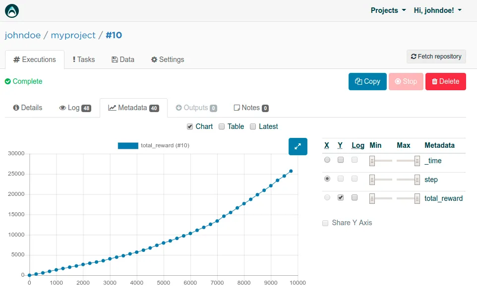
At last we can see some real Q-learning taking place!
After the slow start with high exploration rate, our Q-table is filled with the right data and we reach almost double the total rewards compared to our other agents.
Parallel Executions
So far we have run a single execution at a time, which doesn’t really scale well if you want to iterate fast with your model exploration. For our final effort, instead of one-off executions, we will take our first shot at running a Valohai task. A task in Valohai simply means executing a collection of executions with varying hyperparameters.
Switch to the Tasks tab in Valohai, then click the blue Create task button.
Let’s see how learning_rate parameter affects our performance. Choose Multiple and then type in three different options (0.01, 0.1, 0.25) on different rows. Finally click the blue Create task from the bottom to start executing.
Valohai will now start not one but three server instances in parallel. Each of those boxes with a number inside represent a running instance with a different learning_rate. Once the colour turns to green, it means the execution has finished. You can also view the metadata graph live, while the the executions are running!
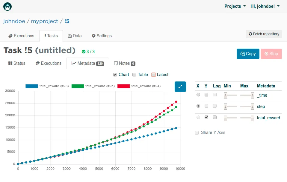
Here are the rewards for three different values for learning_rate . Seems like our original 0.1 performed slightly better than 0.25. Using 0.01 is clearly worse and seems to not learn anything at all for 10000 iterations.
In third part , we will move our Q-learning approach from a Q-table to a deep neural net. Go ahead and read it too!