In part 1 we introduced Q-learning as a concept with a pen and paper example.
In part 2 we implemented the example in code and demonstrated how to execute it in the cloud.
In this third part, we will move our Q-learning approach from a Q-table to a deep neural net.
With Q-table, your memory requirement is an array of states x actions . For the state-space of 5 and action-space of 2, the total memory consumption is 2 x 5=10. But just the state-space of chess is around 10^120, which means this strict spreadsheet approach will not scale to the real world. Luckily you can steal a trick from the world of media compression: Trade some accuracy for memory.
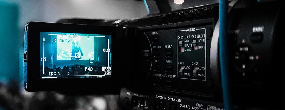
Storing 1080p video at 60 frames per second takes around 1 gigabyte PER SECOND with lossless compression. The same video using a lossy compression can easily be 1/10000th of size without losing much fidelity. Lucky for us, just like with video files, training a model with reinforcement learning is never about 100% fidelity, and something “good enough” or “better than human level” makes the data scientist smile already. Hence we are quite happy with trading accuracy for memory.
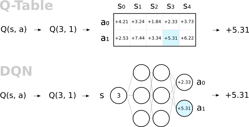
Instead of taking a “perfect” value from our Q-table, we train a neural net to estimate the table. After all, a neural net is nothing more than a glorified table of weights and biases itself!
Our example game is of such simplicity, that we will actually use more memory with the neural net than with the Q-table! Any real world scenario is much more complicated than this, so it is simply an artifact of our attempt to keep the example simple, not a general trend.
Training
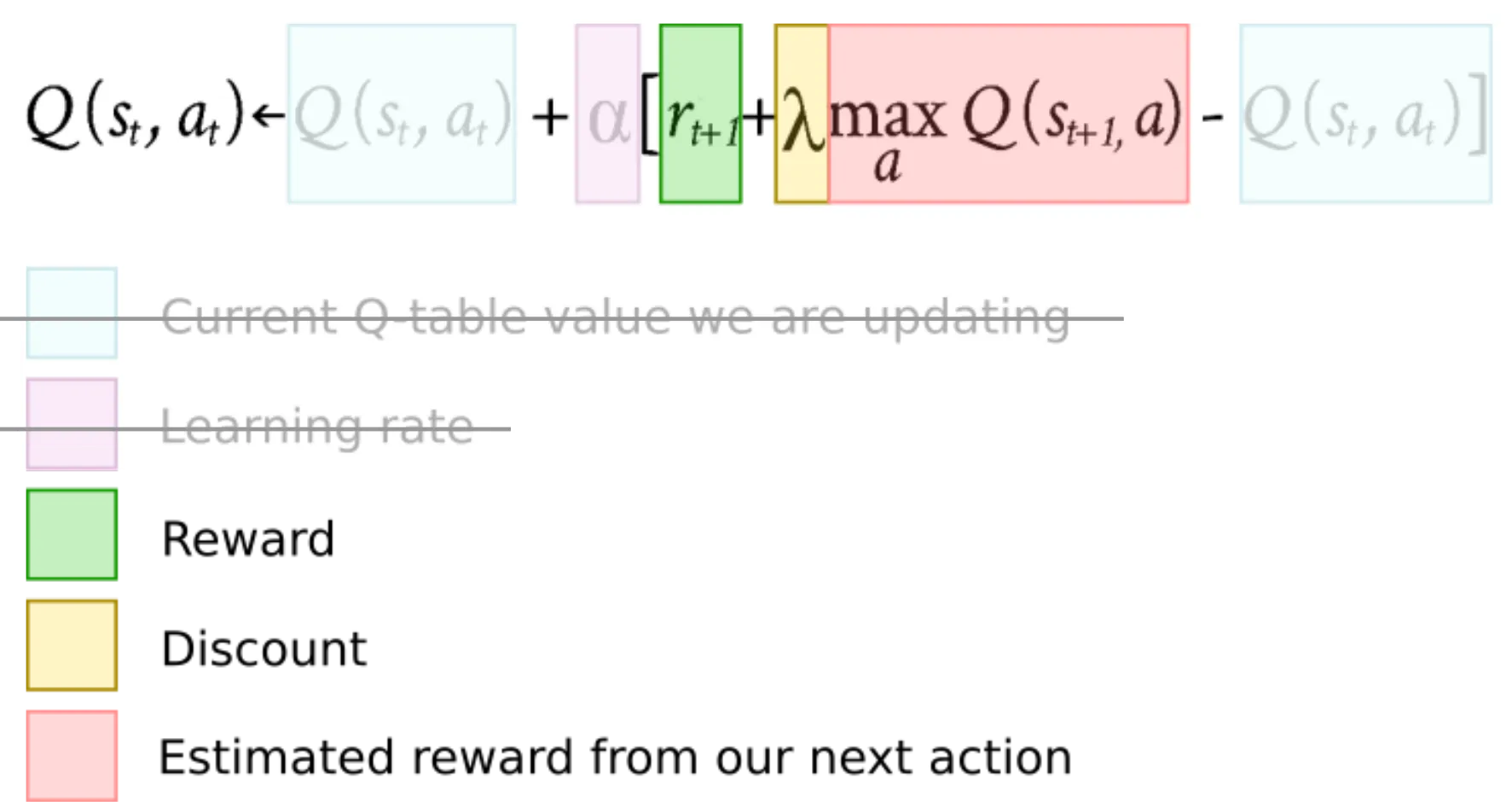
When we did Q-learning earlier, we used the algorithm above. With the neural network taking the place of the Q-table, we can simplify it.
The learning rate is no longer needed, as our back-propagating optimizer will already have that. Learning rate is simply a global gas pedal and one does not need two of those. Once the learning rate is removed, you realize that you can also remove the two Q(s, a) terms, as they cancel each other out after getting rid of the learning rate.
Reinforcement learning is often described as a separate category from supervised and unsupervised learning, yet here we will borrow something from our supervised cousin. Reinforcement learning is said to need no training data, but that is only partly true. Training data is not needed beforehand, but it is collected while exploring the simulation and used quite similarly.
When the agent is exploring the simulation, it will record experiences.
Single experience = (old state, action, reward, new state)
Training our model with a single experience:
-
Let the model estimate Q values of the old state
-
Let the model estimate Q values of the new state
-
Calculate the new target Q value for the action, using the known reward
-
Train the model with input = (old state), output = (target Q values)
Note: Our network doesn’t get (state, action) as input like the Q-learning function Q(s,a) does. This is because we are not replicating Q-learning as a whole, just the Q-table. The input is just the state and the output is Q-values for all possible actions (forward, backward) for that state.
The Code
In the previous part, we were smart enough to separate agent(s), simulation and orchestration as separate classes. This means we can just introduce a new agent and the rest of the code will stay basically the same. If you want to see the rest of the code, see part 2 or the GitHub repo.
Batching
In our example, we retrain the model after each step of the simulation, with just one experience at a time. This is to keep the code simple. This approach is often called online training.
A more common approach is to collect all (or many) of the experiences into a memory log. The model is then trained against multiple random experiences pulled from the log as a batch. This is called batch training or mini-batch training . It is more efficient and often provides more stable training results overall to reinforcement learning. It is quite easy to translate this example into a batch training, as the model inputs and outputs are already shaped to support that.
Results
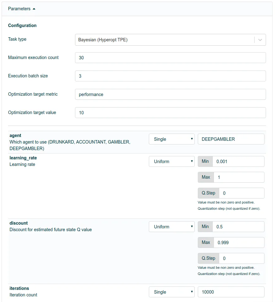
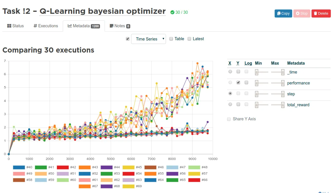
 Here are some training runs with different learning rates and discounts. Note that here we are measuring performance and not total rewards like we did in the previous parts. The upward trend is the result of two things: Learning and exploitation. Learning means the model is learning to minimize the loss and maximize the rewards like usual. Exploitation means that since we start by gambling and exploring and shift linearly towards exploitation more and more, we get better results toward the end, assuming the learned strategy has started to make any sense along the way.
Training a toy simulation like this with a deep neural network is not optimal by any means. The simulation is not very nuanced, the reward mechanism is very coarse and deep networks generally thrive in more complex scenarios. Often in machine learning, the simplest solution ends up being the best one, so cracking a nut with a sledgehammer as we have done here is not recommended in real life.
Now that we have learned how to replace Q-table with a neural network, we are all set to tackle more complicated simulations and utilize the Valohai deep learning platform to the fullest in the next part. I know that Q learning needs a beefy GPU. Valohai has them! You can contact me on LinkedIn about how to get your project started, s ee you soon!
